New Home of Systematic Investor Blog

Please visit the New Home of Systematic Investor Blog at SystematicInvestor.GitHub.io

Adjusted Momentum

David Varadi has published two excellent posts / ideas about cooking with momentum:

• VIX-Adjusted Momentum
• Error-Adjusted Momentum

I just could not resist the urge to share these ideas with you. Following is implementation using the Systematic Investor Toolbox.

###############################################################################
# Load Systematic Investor Toolbox (SIT)
# https://systematicinvestor.wordpress.com/systematic-investor-toolbox/
###############################################################################
setInternet2(TRUE)
con = gzcon(url('http://www.systematicportfolio.com/sit.gz', 'rb'))
    source(con)
close(con)
	#*****************************************************************
	# Load historical data
	#****************************************************************** 
	load.packages('quantmod')
		
	tickers = spl('SPY,^VIX')
		
	data <- new.env()
	getSymbols(tickers, src = 'yahoo', from = '1980-01-01', env = data, auto.assign = T)
		for(i in data$symbolnames) data[[i]] = adjustOHLC(data[[i]], use.Adjusted=T)
	bt.prep(data, align='remove.na', fill.gaps = T)

	VIX = Cl(data$VIX)
	bt.prep.remove.symbols(data, 'VIX')
	
	#*****************************************************************
	# Setup
	#*****************************************************************
	prices = data$prices
		
	models = list()

	#*****************************************************************
	# 200 SMA
	#****************************************************************** 
	data$weight[] = NA
		data$weight[] = iif(prices > SMA(prices, 200), 1, 0)
	models$ma200 = bt.run.share(data, clean.signal=T)
	
	#*****************************************************************
	# 200 ROC
	#****************************************************************** 
	roc = prices / mlag(prices) - 1
	
	data$weight[] = NA
		data$weight[] = iif(SMA(roc, 200) > 0, 1, 0)
	models$roc200 = bt.run.share(data, clean.signal=T)
	
	#*****************************************************************
	# 200 VIX MOM
	#****************************************************************** 
	data$weight[] = NA
		data$weight[] = iif(SMA(roc/VIX, 200) > 0, 1, 0)
	models$vix.mom = bt.run.share(data, clean.signal=T)

	#*****************************************************************
	# 200 ER MOM
	#****************************************************************** 
	forecast = SMA(roc,10)
	error = roc - mlag(forecast)
	mae = SMA(abs(error), 10)
	
	data$weight[] = NA
		data$weight[] = iif(SMA(roc/mae, 200) > 0, 1, 0)
	models$er.mom = bt.run.share(data, clean.signal=T)
		
	#*****************************************************************
	# Report
	#****************************************************************** 
	strategy.performance.snapshoot(models, T)

Please enjoy and share your ideas with David and myself.

To view the complete source code for this example, please have a look at the
bt.adjusted.momentum.test() function in bt.test.r at github.

Calendar Strategy: Fed Days

UPDATE: I was pointed out a problem with original post due to look ahead bias introduced by prices > SMA(prices,100) statement. In the calendar strategy logic I did not use a usual lag of one day because important days are known before hand. However, the prices > SMA(prices,100) statement should be lagged by one day. I updated plots and source code.

Today, I want to follow up with the Calendar Strategy: Option Expiry post. Let’s examine the importance of the FED meeting days as presented in the Fed Days And Intermediate-Term Highs post.

Let’s dive in and examine historical perfromance of SPY during FED meeting days:

###############################################################################
# Load Systematic Investor Toolbox (SIT)
# https://systematicinvestor.wordpress.com/systematic-investor-toolbox/
###############################################################################
setInternet2(TRUE)
con = gzcon(url('http://www.systematicportfolio.com/sit.gz', 'rb'))
    source(con)
close(con)
	#*****************************************************************
	# Load historical data
	#****************************************************************** 
	load.packages('quantmod')
		
	tickers = spl('SPY')
		
	data <- new.env()
	getSymbols.extra(tickers, src = 'yahoo', from = '1980-01-01', env = data, set.symbolnames = T, auto.assign = T)
		for(i in data$symbolnames) data[[i]] = adjustOHLC(data[[i]], use.Adjusted=T)
	bt.prep(data, align='keep.all', fill.gaps = T)

	#*****************************************************************
	# Setup
	#*****************************************************************
	prices = data$prices
		n = ncol(prices)
		
	dates = data$dates	
	
	models = list()
	
	universe = prices > 0
		# 100 day SMA filter
		universe = universe & prices > SMA(prices,100)
		
	# Find Fed Days
	info = get.FOMC.dates(F)
		key.date.index = na.omit(match(info$day, dates))
	
	key.date = NA * prices
		key.date[key.date.index,] = T
		
	#*****************************************************************
	# Strategy
	#*****************************************************************
	signals = list(T0=0)
		for(i in 1:15) signals[[paste0('N',i)]] = 0:i	
	signals = calendar.signal(key.date, signals)
	models = calendar.strategy(data, signals, universe = universe)

	strategy.performance.snapshoot(models, T, sort.performance=F)

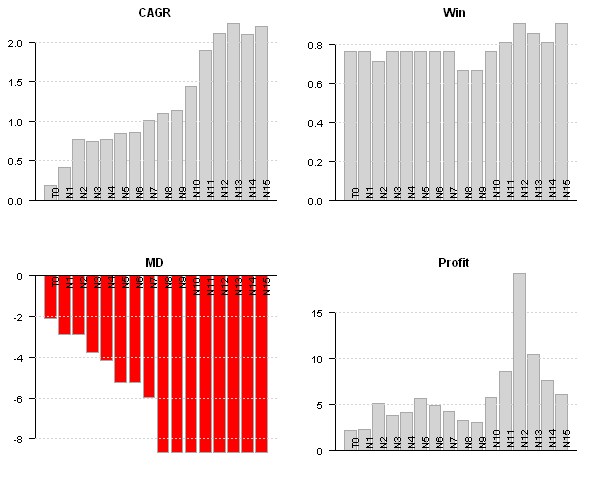
Please note 100 day moving average filter above. If we take it out, the performance deteriorates significantly.

	# custom stats	
	out = sapply(models, function(x) list(
		CAGR = 100*compute.cagr(x$equity),
		MD = 100*compute.max.drawdown(x$equity),
		Win = x$trade.summary$stats['win.prob', 'All'],
		Profit = x$trade.summary$stats['profitfactor', 'All']
		))	
	performance.barchart.helper(out, sort.performance = F)
	
	strategy.performance.snapshoot(models$N15, control=list(main=T))
	
	last.trades(models$N15)
	
	trades = models$N15$trade.summary$trades
		trades = make.xts(parse.number(trades[,'return']), as.Date(trades[,'entry.date']))
	layout(1:2)
		par(mar = c(4,3,3,1), cex = 0.8) 
	barplot(trades, main='N15 Trades', las=1)
	plot(cumprod(1+trades/100), type='b', main='N15 Trades', las=1)

N15 Strategy:

With this post I wanted to show how easily we can study calendar strategy performance using the Systematic Investor Toolbox.

Next, I will look at the importance of the Dividend days.

To view the complete source code for this example, please have a look at the bt.calendar.strategy.fed.days.test() function in bt.test.r at github.

Calendar Strategy: Option Expiry

Today, I want to follow up with the Calendar Strategy: Month End post. Let’s examine the perfromance Option Expiry days as presented in the The Mooost Wonderful Tiiiiiiime of the Yearrrrrrrrr! post.

First, I created two convenience functions for creating a calendar signal and back-testing calendar strategy: calendar.signal and calendar.strategy functions are in the strategy.r at github

Now, let’s dive in and examine historical perfromance of SPY during Option Expiry period in December:

###############################################################################
# Load Systematic Investor Toolbox (SIT)
# https://systematicinvestor.wordpress.com/systematic-investor-toolbox/
###############################################################################
setInternet2(TRUE)
con = gzcon(url('http://www.systematicportfolio.com/sit.gz', 'rb'))
    source(con)
close(con)

	#*****************************************************************
	# Load historical data
	#****************************************************************** 
	load.packages('quantmod')
		
	tickers = spl('SPY')
		
	data <- new.env()
	getSymbols.extra(tickers, src = 'yahoo', from = '1980-01-01', env = data, set.symbolnames = T, auto.assign = T)
		for(i in data$symbolnames) data[[i]] = adjustOHLC(data[[i]], use.Adjusted=T)
	bt.prep(data, align='keep.all', fill.gaps = T)

	#*****************************************************************
	# Setup
	#*****************************************************************
	prices = data$prices
		n = ncol(prices)
		
	dates = data$dates	
	
	models = list()
	
	universe = prices > 0
		
	# Find Friday before options expiration week in December
	years = date.year(range(dates))
	second.friday = third.friday.month(years[1]:years[2], 12) - 7
		key.date.index = na.omit(match(second.friday, dates))
				
	key.date = NA * prices
		key.date[key.date.index,] = T

	#*****************************************************************
	# Strategy: Op-ex week in December most bullish week of the year for the SPX
	#   Buy: December Friday prior to op-ex.
	#   Sell X days later: 100K/trade 1984-present
	# http://quantifiableedges.blogspot.com/2011/12/mooost-wonderful-tiiiiiiime-of.html
	#*****************************************************************
	signals = list(T0=0)
		for(i in 1:15) signals[[paste0('N',i)]] = 0:i	
	signals = calendar.signal(key.date, signals)
	models = calendar.strategy(data, signals, universe = universe)
	    
	strategy.performance.snapshoot(models, T, sort.performance=F)

Strategies vary in perfromance, next let’s examine a bit more details

	# custom stats	
	out = sapply(models, function(x) list(
		CAGR = 100*compute.cagr(x$equity),
		MD = 100*compute.max.drawdown(x$equity),
		Win = x$trade.summary$stats['win.prob', 'All'],
		Profit = x$trade.summary$stats['profitfactor', 'All']
		))	
	performance.barchart.helper(out, sort.performance = F)
	
	# Plot 15 day strategy
	strategy.performance.snapshoot(models$N15, control=list(main=T))
	
	# Plot trades for 15 day strategy
	last.trades(models$N15)
	
	# Make a summary plot of trades for 15 day strategy
	trades = models$N15$trade.summary$trades
		trades = make.xts(parse.number(trades[,'return']), as.Date(trades[,'entry.date']))
	layout(1:2)
		par(mar = c(4,3,3,1), cex = 0.8) 
	barplot(trades, main='Trades', las=1)
	plot(cumprod(1+trades/100), type='b', main='Trades', las=1)

Details for the 15 day strategy:

With this post I wanted to show how easily we can study calendar strategy performance using the Systematic Investor Toolbox.

Next, I will look at the importance of the FED meeting days.

To view the complete source code for this example, please have a look at the
bt.calendar.strategy.option.expiry.test() function in bt.test.r at github.

Calendar Strategy: Month End

Calendar Strategy is a very simple strategy that buys an sells at the predetermined days, known in advance. Today I want to show how we can easily investigate performance at and around Month End days.

First let’s load historical prices for SPY from Yahoo Fiance and compute SPY perfromance at the month-ends. I.e. strategy will open long position at the close on the 30th and sell position at the close on the 31st.

###############################################################################
# Load Systematic Investor Toolbox (SIT)
# https://systematicinvestor.wordpress.com/systematic-investor-toolbox/
###############################################################################
setInternet2(TRUE)
con = gzcon(url('http://www.systematicportfolio.com/sit.gz', 'rb'))
    source(con)
close(con)
	#*****************************************************************
	# Load historical data
	#****************************************************************** 
	load.packages('quantmod')
		
	tickers = spl('SPY')
		
	data <- new.env()
	getSymbols.extra(tickers, src = 'yahoo', from = '1980-01-01', env = data, set.symbolnames = T, auto.assign = T)
		for(i in data$symbolnames) data[[i]] = adjustOHLC(data[[i]], use.Adjusted=T)
	bt.prep(data, align='keep.all', fill.gaps = T)

	#*****************************************************************
	# Setup
	#*****************************************************************
	prices = data$prices
		n = ncol(prices)
		
	models = list()
		
	period.ends = date.month.ends(data$dates, F)
		
	#*****************************************************************
	# Strategy
	#*****************************************************************
	key.date = NA * prices
		key.date[period.ends] = T
	
	universe = prices > 0
	signal = key.date

	data$weight[] = NA
		data$weight[] = ifna(universe & key.date, F)
	models$T0 = bt.run.share(data, do.lag = 0, trade.summary=T, clean.signal=T) 

Please note that above, in the bt.run.share call, I set do.lag parameter equal to zero (the default value for the do.lag parameter is one). The reason for default setting equal to one is due to signal (decision to trade) is derived using all information available today, so the position can only be implement next day. I.e.

portfolio.returns = lag(signal, do.lag) * returns = lag(signal, 1) * returns

However, in case of the calendar strategy there is no need to lag signal because the trade day is known in advance. I.e.

portfolio.returns = lag(signal, do.lag) * returns = signal * returns

Next, I created two functions to help with signal creation and strategy testing:

	calendar.strategy <- function(data, signal, universe = data$prices > 0) {
		data$weight[] = NA
			data$weight[] = ifna(universe & signal, F)
		bt.run.share(data, do.lag = 0, trade.summary=T, clean.signal=T)  	
	}
	
	calendar.signal <- function(key.date, offsets = 0) {
		signal = mlag(key.date, offsets[1])
		for(i in offsets) signal = signal | mlag(key.date, i)
		signal
	}

	# Trade on key.date
	models$T0 = calendar.strategy(data, key.date)

	# Trade next day after key.date
	models$N1 = calendar.strategy(data, mlag(key.date,1))
	# Trade two days next(after) key.date
	models$N2 = calendar.strategy(data, mlag(key.date,2))

	# Trade a day prior to key.date
	models$P1 = calendar.strategy(data, mlag(key.date,-1))
	# Trade two days prior to key.date
	models$P2 = calendar.strategy(data, mlag(key.date,-2))
	
	# Trade: open 2 days before the key.date and close 2 days after the key.date
	signal = key.date | mlag(key.date,-1) | mlag(key.date,-2) | mlag(key.date,1) | mlag(key.date,2)
	models$P2N2 = calendar.strategy(data, signal)

	# same, but using helper function above	
	models$P2N2 = calendar.strategy(data, calendar.signal(key.date, -2:2))
		
	strategy.performance.snapshoot(models, T)
	
	strategy.performance.snapshoot(models, control=list(comparison=T), sort.performance=F)

Above, T0 is a calendar strategy that buys on 30th and sells on 31st. I.e. position is only held on a month end day. P1 and P2 are two strategies that buy a day prior and two days prior correspondingly. N1 and N2 are two strategies that buy a day after and two days after correspondingly.

The N1 strategy, buy on 31st and sell on the 1st next month seems to be working best for SPY.

Finally, let’s look at the actual trades:

	last.trades <- function(model, n=20, make.plot=T, return.table=F) {
		ntrades = min(n, nrow(model$trade.summary$trades))		
		trades = last(model$trade.summary$trades, ntrades)
		if(make.plot) {
			layout(1)
			plot.table(trades)
		}	
		if(return.table) trades	
	}
	
	last.trades(models$P2)

The P2 strategy enters position at the close 3 days before the month end and exits positions at the close 2 days before the month end. I.e. the performance is due to returns only 2 days before the month end.

With this post I wanted to show how easily we can study calendar strategy performance using the Systematic Investor Toolbox.

Next, I will demonstrate calendar strategy applications to variety of important dates.

To view the complete source code for this example, please have a look at the bt.calendar.strategy.month.end.test() function in bt.test.r at github.