Archive
Adjusted Momentum
David Varadi has published two excellent posts / ideas about cooking with momentum:
I just could not resist the urge to share these ideas with you. Following is implementation using the Systematic Investor Toolbox.
###############################################################################
# Load Systematic Investor Toolbox (SIT)
# https://systematicinvestor.wordpress.com/systematic-investor-toolbox/
###############################################################################
setInternet2(TRUE)
con = gzcon(url('http://www.systematicportfolio.com/sit.gz', 'rb'))
    source(con)
close(con)
	#*****************************************************************
	# Load historical data
	#******************************************************************
	load.packages('quantmod')

	tickers = spl('SPY,^VIX')

	data <- new.env()
	getSymbols(tickers, src = 'yahoo', from = '1980-01-01', env = data, auto.assign = T)
		for(i in data$symbolnames) data[[i]] = adjustOHLC(data[[i]], use.Adjusted=T)
	bt.prep(data, align='remove.na', fill.gaps = T)

	VIX = Cl(data$VIX)
	bt.prep.remove.symbols(data, 'VIX')

	#*****************************************************************
	# Setup
	#*****************************************************************
	prices = data$prices

	models = list()

	#*****************************************************************
	# 200 SMA
	#******************************************************************
	data$weight[] = NA
		data$weight[] = iif(prices > SMA(prices, 200), 1, 0)
	models$ma200 = bt.run.share(data, clean.signal=T)

	#*****************************************************************
	# 200 ROC
	#******************************************************************
	roc = prices / mlag(prices) - 1

	data$weight[] = NA
		data$weight[] = iif(SMA(roc, 200) > 0, 1, 0)
	models$roc200 = bt.run.share(data, clean.signal=T)

	#*****************************************************************
	# 200 VIX MOM
	#******************************************************************
	data$weight[] = NA
		data$weight[] = iif(SMA(roc/VIX, 200) > 0, 1, 0)
	models$vix.mom = bt.run.share(data, clean.signal=T)

	#*****************************************************************
	# 200 ER MOM
	#******************************************************************
	forecast = SMA(roc,10)
	error = roc - mlag(forecast)
	mae = SMA(abs(error), 10)

	data$weight[] = NA
		data$weight[] = iif(SMA(roc/mae, 200) > 0, 1, 0)
	models$er.mom = bt.run.share(data, clean.signal=T)

	#*****************************************************************
	# Report
	#******************************************************************
	strategy.performance.snapshoot(models, T)

Please enjoy and share your ideas with David and myself.
To view the complete source code for this example, please have a look at the
bt.adjusted.momentum.test() function in bt.test.r at github.
Probabilistic Momentum
David Varadi has recently discussed an interesting strategy in the
Are Simple Momentum Strategies Too Dumb? Introducing Probabilistic Momentum post. David also provided the Probabilistic Momentum Spreadsheet if you are interested in doing computations in Excel. Today I want to show how you can test such strategy using the Systematic Investor Toolbox:
###############################################################################
# Load Systematic Investor Toolbox (SIT)
# https://systematicinvestor.wordpress.com/systematic-investor-toolbox/
###############################################################################
setInternet2(TRUE)
con = gzcon(url('http://www.systematicportfolio.com/sit.gz', 'rb'))
    source(con)
close(con)
	#*****************************************************************
	# Load historical data
	#******************************************************************
	load.packages('quantmod')

	tickers = spl('SPY,TLT')

	data <- new.env()
	getSymbols(tickers, src = 'yahoo', from = '1980-01-01', env = data, auto.assign = T)
		for(i in ls(data)) data[[i]] = adjustOHLC(data[[i]], use.Adjusted=T)
	bt.prep(data, align='remove.na', dates='2005::')


	#*****************************************************************
	# Setup
	#******************************************************************
	lookback.len = 60

	prices = data$prices

	models = list()

	#*****************************************************************
	# Simple Momentum
	#******************************************************************
	momentum = prices / mlag(prices, lookback.len)
	data$weight[] = NA
		data$weight$SPY[] = momentum$SPY > momentum$TLT
		data$weight$TLT[] = momentum$SPY <= momentum$TLT
	models$Simple  = bt.run.share(data, clean.signal=T)
The Simple Momentum strategy invests into SPY if SPY’s momentum if greater than TLT’s momentum, and invests into TLT otherwise.
	#*****************************************************************
	# Probabilistic Momentum
	#******************************************************************
	confidence.level = 60/100
	ret = prices / mlag(prices) - 1

	ir = sqrt(lookback.len) * runMean(ret$SPY - ret$TLT, lookback.len) / runSD(ret$SPY - ret$TLT, lookback.len)
	momentum.p = pt(ir, lookback.len - 1)

	data$weight[] = NA
		data$weight$SPY[] = iif(cross.up(momentum.p, confidence.level), 1, iif(cross.dn(momentum.p, (1 - confidence.level)), 0,NA))
		data$weight$TLT[] = iif(cross.dn(momentum.p, (1 - confidence.level)), 1, iif(cross.up(momentum.p, confidence.level), 0,NA))
	models$Probabilistic  = bt.run.share(data, clean.signal=T)
The Probabilistic Momentum strategy is using Probabilistic Momentum measure and Confidence Level to decide on allocation. Strategy invests into SPY if SPY vs TLT Probabilistic Momentum is above Confidence Level and invests into TLT is SPY vs TLT Probabilistic Momentum is below 1 – Confidence Level.
To make Strategy a bit more attractive, I added a version that can leverage SPY allocation by 50%
	#*****************************************************************
	# Probabilistic Momentum + SPY Leverage
	#******************************************************************
	data$weight[] = NA
		data$weight$SPY[] = iif(cross.up(momentum.p, confidence.level), 1, iif(cross.up(momentum.p, (1 - confidence.level)), 0,NA))
		data$weight$TLT[] = iif(cross.dn(momentum.p, (1 - confidence.level)), 1, iif(cross.up(momentum.p, confidence.level), 0,NA))
	models$Probabilistic.Leverage = bt.run.share(data, clean.signal=T)

	#*****************************************************************
	# Create Report
	#******************************************************************
	strategy.performance.snapshoot(models, T)

The back-test results look very similar to the ones reported in the Are Simple Momentum Strategies Too Dumb? Introducing Probabilistic Momentum post.
However, I was not able to exactly reproduce the transition plots. Looks like my interpretation is producing more whipsaw when desired.
	#*****************************************************************
	# Visualize Signal
	#******************************************************************
	cols = spl('steelblue1,steelblue')
	prices = scale.one(data$prices)

	layout(1:3)

	plota(prices$SPY, type='l', ylim=range(prices), plotX=F, col=cols[1], lwd=2)
	plota.lines(prices$TLT, type='l', plotX=F, col=cols[2], lwd=2)
		plota.legend('SPY,TLT',cols,as.list(prices))

	highlight = models$Probabilistic$weight$SPY > 0
		plota.control$col.x.highlight = iif(highlight, cols[1], cols[2])
	plota(models$Probabilistic$equity, type='l', plotX=F, x.highlight = highlight | T)
		plota.legend('Probabilistic,SPY,TLT',c('black',cols))

	highlight = models$Simple$weight$SPY > 0
		plota.control$col.x.highlight = iif(highlight, cols[1], cols[2])
	plota(models$Simple$equity, type='l', plotX=T, x.highlight = highlight | T)
		plota.legend('Simple,SPY,TLT',c('black',cols))

David thank you very much for sharing your great ideas. I would encourage readers to play with this strategy and report back.
To view the complete source code for this example, please have a look at the bt.probabilistic.momentum.test() function in bt.test.r at github.
Stochastic Oscillator
I came across the link to the John Ehlers paper: Predictive Indicators for Effective Trading Strategies, while reading the Dekalog Blog. John Ehlers offers a different way to smooth prices and incorporate the new filter into the oscillator construction. Fortunately, the EasyLanguage code was also provided and i was able to translate it into R.
Following are some results from the paper and test of John’s stochastic oscillator.
###############################################################################
# Super Smoother filter 2013 John F. Ehlers
# http://www.stockspotter.com/files/PredictiveIndicators.pdf
###############################################################################
super.smoother.filter <- function(x) {
    a1 = exp( -1.414 * pi / 10.0 )
    b1 = 2.0 * a1 * cos( (1.414*180.0/10.0) * pi / 180.0 )
    c2 = b1
    c3 = -a1 * a1
    c1 = 1.0 - c2 - c3

    x = c1 * (x + mlag(x)) / 2
        x[1] = x[2]

    out = x * NA
        out[] = filter(x, c(c2, c3), method='recursive', init=c(0,0))
    out
}

# Roofing filter 2013 John F. Ehlers
roofing.filter <- function(x) {
    # Highpass filter cyclic components whose periods are shorter than 48 bars
    alpha1 = (cos((0.707*360 / 48) * pi / 180.0 ) + sin((0.707*360 / 48) * pi / 180.0 ) - 1) / cos((0.707*360 / 48) * pi / 180.0 )

    x = (1 - alpha1 / 2)*(1 - alpha1 / 2)*( x - 2*mlag(x) + mlag(x,2))
        x[1] = x[2] = x[3]

    HP = x * NA
    HP[] = filter(x, c(2*(1 - alpha1), - (1 - alpha1)*(1 - alpha1)), method='recursive', init=c(0,0))

    super.smoother.filter(HP)
}

# My Stochastic Indicator 2013 John F. Ehlers
roofing.stochastic.indicator  <- function(x, lookback = 20) {
    Filt = roofing.filter(x)

    HighestC = runMax(Filt, lookback)
        HighestC[1:lookback] = as.double(HighestC[lookback])
    LowestC = runMin(Filt, lookback)
        LowestC[1:lookback] = as.double(LowestC[lookback])
    Stoc = (Filt - LowestC) / (HighestC - LowestC)

    super.smoother.filter(Stoc)
}
First let’s plot the John’s stochastic oscillator vs traditional one.
###############################################################################
# Load Systematic Investor Toolbox (SIT)
# https://systematicinvestor.wordpress.com/systematic-investor-toolbox/
###############################################################################
setInternet2(TRUE)
con = gzcon(url('http://www.systematicportfolio.com/sit.gz', 'rb'))
    source(con)
close(con)

    #*****************************************************************
    # Load historical data
    #******************************************************************
    load.packages('quantmod')

    tickers = spl('DG')
    data = new.env()
    getSymbols(tickers, src = 'yahoo', from = '1970-01-01', env = data, auto.assign = T)
        for(i in ls(data)) data[[i]] = adjustOHLC(data[[i]], use.Adjusted=T)
    bt.prep(data)

    #*****************************************************************
    # Setup
    #*****************************************************************
    prices = data$prices

    models = list()

    # John Ehlers Stochastic
    stoch = roofing.stochastic.indicator(prices)

    # 14 Day Stochastic
    stoch14 = bt.apply(data, function(x) stoch(HLC(x),14)[,'slowD'])

    #*****************************************************************
    # Create plots
    #******************************************************************
    dates = '2011:10::2012:9'

    layout(1:3)

    plota(prices[dates], type='l', plotX=F)
    plota.legend('DG')

    plota(stoch[dates], type='l', plotX=F)
        abline(h = 0.2, col='red')
        abline(h = 0.8, col='red')
    plota.legend('John Ehlers Stochastic')

    plota(stoch14[dates], type='l')
        abline(h = 0.2, col='red')
        abline(h = 0.8, col='red')
    plota.legend('Stochastic')

Next let’s code the trading rules as in Figure 6 and 8 in the John Ehlers paper: Predictive Indicators for Effective Trading Strategies
    #*****************************************************************
    # Code Strategies
    #*****************************************************************
    # Figure 6: Conventional Wisdom is to Buy When the Indicator Crosses Above 20% and
    # To Sell Short when the Indicator Crosses below 80%
    data$weight[] = NA
        data$weight[] = iif(cross.up(stoch, 0.2), 1, iif(cross.dn(stoch, 0.8), -1, NA))
    models$post = bt.run.share(data, clean.signal=T, trade.summary=T)

    data$weight[] = NA
        data$weight[] = iif(cross.up(stoch, 0.2), 1, iif(cross.dn(stoch, 0.8), 0, NA))
    models$post.L = bt.run.share(data, clean.signal=T, trade.summary=T)

    data$weight[] = NA
        data$weight[] = iif(cross.up(stoch, 0.2), 0, iif(cross.dn(stoch, 0.8), -1, NA))
    models$post.S = bt.run.share(data, clean.signal=T, trade.summary=T)

    # Figure 8: Predictive Indicators Enable You to Buy When the Indicator Crosses Below 20% and
    # To Sell Short when the Indicator Crosses Above 80%
    data$weight[] = NA
        data$weight[] = iif(cross.dn(stoch, 0.2), 1, iif(cross.up(stoch, 0.8), -1, NA))
    models$pre = bt.run.share(data, clean.signal=T, trade.summary=T)

    data$weight[] = NA
        data$weight[] = iif(cross.dn(stoch, 0.2), 1, iif(cross.up(stoch, 0.8), 0, NA))
    models$pre.L = bt.run.share(data, clean.signal=T, trade.summary=T)

    data$weight[] = NA
        data$weight[] = iif(cross.dn(stoch, 0.2), 0, iif(cross.up(stoch, 0.8), -1, NA))
    models$pre.S = bt.run.share(data, clean.signal=T, trade.summary=T)

    #*****************************************************************
    # Create Report
    #******************************************************************
    strategy.performance.snapshoot(models, T)

Look’s like most profit comes from the long side.
Finally let’s visualize the timing of the signal for these strategies:
john.ehlers.custom.strategy.plot <- function(data, models, name,
	main = name,
	dates = '::',
	layout = NULL		# flag to indicate if layout is already set
) {
    # John Ehlers Stochastic
    stoch = roofing.stochastic.indicator(data$prices)

    # highlight logic based on weight
    weight = models[[name]]$weight[dates]
    	col = iif(weight > 0, 'green', iif(weight < 0, 'red', 'white'))
    plota.control$col.x.highlight = col.add.alpha(col, 100)
    	highlight = T

    if(is.null(layout)) layout(1:2)

    plota(data$prices[dates], type='l', x.highlight = highlight, plotX = F, main=main)
    plota.legend('Long,Short,Not Invested','green,red,white')

    plota(stoch[dates], type='l', x.highlight = highlight, plotX = F, ylim=c(0,1))
       	col = col.add.alpha('red', 100)
        abline(h = 0.2, col=col, lwd=3)
        abline(h = 0.8, col=col, lwd=3)
    plota.legend('John Ehlers Stochastic')
}


    layout(1:4, heights=c(2,1,2,1))

    john.ehlers.custom.strategy.plot(data, models, 'post.L', dates = '2013::', layout=T,
        main = 'post.L: Buy When the Indicator Crosses Above 20% and Sell when the Indicator Crosses Below 80%')

    john.ehlers.custom.strategy.plot(data, models, 'pre.L', dates = '2013::', layout=T,
	main = 'pre.L: Buy When the Indicator Crosses Below 20% and Sell when the Indicator Crosses Above 80%')

As a homework, I encourage you to compare trading the John’s stochastic oscillator vs traditional one.
To view the complete source code for this example, please have a look at the john.ehlers.filter.test() function in bt.test.r at github.
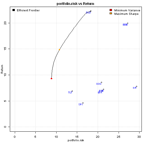
Maximum Sharpe Portfolio
Maximum Sharpe Portfolio or Tangency Portfolio is a portfolio on the efficient frontier at the point where line drawn from the point (0, risk-free rate) is tangent to the efficient frontier.
There is a great discussion about Maximum Sharpe Portfolio or Tangency Portfolio at quadprog optimization question. In general case, finding the Maximum Sharpe Portfolio requires a non-linear solver because we want to find portfolio weights w to maximize w' mu / sqrt( w' V w ) (i.e. Sharpe Ratio is a non-linear function of w). But as discussed in the quadprog optimization question, there are special cases when we can use quadratic solver to find Maximum Sharpe Portfolio. As long as all constraints are homogeneous of degree 0 (i.e. if we multiply w by a number, the constraint is unchanged – for example, w1 > 0 is equivalent to 5*w1 > 5*0), the quadratic solver can be used to find Maximum Sharpe Portfolio or Tangency Portfolio.
I have implemented the logic to find Maximum Sharpe Portfolio or Tangency Portfolio in the max.sharpe.portfolio() function in strategy.r at github. You can specify following 2 parameters:
- Type of portfolio: ‘long-only’, ‘long-short’, or ‘market-neutral’
- Portfolio exposure. For example, ‘long-only’ with exposure = 1, is a fully invested portfolio
Now, let’s construct a sample efficient frontier and plot Maximum Sharpe Portfolio.
###############################################################################
# Load Systematic Investor Toolbox (SIT)
# https://systematicinvestor.wordpress.com/systematic-investor-toolbox/
###############################################################################
setInternet2(TRUE)
con = gzcon(url('http://www.systematicportfolio.com/sit.gz', 'rb'))
    source(con)
close(con)

	#*****************************************************************
	# Create Efficient Frontier
	#******************************************************************
	# create sample historical input assumptions
	ia = aa.test.create.ia()

	# create long-only, fully invested efficient frontier
	n = ia$n

	# 0 <= x.i <= 1
	constraints = new.constraints(n, lb = 0, ub = 1)
		constraints = add.constraints(diag(n), type='>=', b=0, constraints)
		constraints = add.constraints(diag(n), type='<=', b=1, constraints)

	# SUM x.i = 1
	constraints = add.constraints(rep(1, n), 1, type = '=', constraints)

	# create efficient frontier
	ef = portopt(ia, constraints, 50, 'Efficient Frontier')

	#*****************************************************************
	# Create Plot
	#******************************************************************
	# plot efficient frontier
	plot.ef(ia, list(ef), transition.map=F)

	# find maximum sharpe portfolio
	max(portfolio.return(ef$weight,ia) /  portfolio.risk(ef$weight,ia))

	# plot minimum variance portfolio
	weight = min.var.portfolio(ia,constraints)
	points(100 * portfolio.risk(weight,ia), 100 * portfolio.return(weight,ia), pch=15, col='red')
	portfolio.return(weight,ia) /  portfolio.risk(weight,ia)

	# plot maximum Sharpe or tangency portfolio
	weight = max.sharpe.portfolio()(ia,constraints)
	points(100 * portfolio.risk(weight,ia), 100 * portfolio.return(weight,ia), pch=15, col='orange')
	portfolio.return(weight,ia) /  portfolio.risk(weight,ia)

	plota.legend('Minimum Variance,Maximum Sharpe','red,orange', x='topright')
Now let’s see how to construct ‘long-only’, ‘long-short’, or ‘market-neutral’ Maximum Sharpe Portfolio or Tangency Portfolios:
	#*****************************************************************
	# Examples of Maximum Sharpe or Tangency portfolios construction
	#******************************************************************
	weight = max.sharpe.portfolio('long-only')(ia,constraints)
		round(weight,2)
		round(c(sum(weight[weight<0]), sum(weight[weight>0])),2)

	weight = max.sharpe.portfolio('long-short')(ia,constraints)
		round(weight,2)
		round(c(sum(weight[weight<0]), sum(weight[weight>0])),2)

	weight = max.sharpe.portfolio('market-neutral')(ia,constraints)
		round(weight,2)
		round(c(sum(weight[weight<0]), sum(weight[weight>0])),2)
The long-only Maximum Sharpe portfolio as expected has exposure of 100%. The long-short Maximum Sharpe portfolio is 227% long and 127% short. The market-neutral Maximum Sharpe portfolio is 100% long and 100% short.
As the last step, I run Maximum Sharpe algo vs other portfolio optimization methods I have previously discussed (i.e. Risk Parity, Minimum Variance, Maximum Diversification, Minimum Correlation) on the 10 asset universe used in the Adaptive Asset Allocation post.
	#*****************************************************************
	# Load historical data
	#******************************************************************
	load.packages('quantmod')

	tickers = spl('SPY,EFA,EWJ,EEM,IYR,RWX,IEF,TLT,DBC,GLD')

	data <- new.env()
	getSymbols(tickers, src = 'yahoo', from = '1980-01-01', env = data, auto.assign = T)
		for(i in ls(data)) data[[i]] = adjustOHLC(data[[i]], use.Adjusted=T)
	bt.prep(data, align='keep.all', dates='2004:12::')

	#*****************************************************************
	# Code Strategies
	#******************************************************************
	prices = data$prices
	n = ncol(prices)

	models = list()

 	#*****************************************************************
	# Code Strategies
	#******************************************************************
	# find period ends
	period.ends = endpoints(prices, 'months')
        period.ends = period.ends[period.ends > 0]

	n.mom = 180
	n.vol = 60
	n.top = 4
	momentum = prices / mlag(prices, n.mom)

	obj = portfolio.allocation.helper(data$prices, period.ends=period.ends,
		lookback.len = n.vol, universe = ntop(momentum[period.ends,], n.top) > 0,
		min.risk.fns = list(EW=equal.weight.portfolio,
						RP=risk.parity.portfolio,
						MV=min.var.portfolio,
						MD=max.div.portfolio,
						MC=min.corr.portfolio,
						MC2=min.corr2.portfolio,
						MCE=min.corr.excel.portfolio,
						MS=max.sharpe.portfolio())
	)

	models = create.strategies(obj, data)$models

	#*****************************************************************
	# Create Report
	#******************************************************************
	strategy.performance.snapshoot(models, T)

	plotbt.custom.report.part2(models$MS)

	# Plot Portfolio Turnover for each strategy
	layout(1)
	barplot.with.labels(sapply(models, compute.turnover, data), 'Average Annual Portfolio Turnover')
The allocation using Maximum Sharpe Portfolio produced more concentrated portfolios with higher total return, higher Sharpe ratio, and higher turnover.


Modeling Couch Potato strategy
I first read about the Couch Potato strategy in the MoneySense magazine. I liked this simple strategy because it was easy to understand and easy to manage. The Couch Potato strategy is similar to the Permanent Portfolio strategy that I have analyzed previously.
The Couch Potato strategy invests money in the given proportions among different types of assets to ensure diversification and rebalances the holdings once a year. For example the Classic Couch Potato strategy is:
- 1) Canadian equity (33.3%)
- 2) U.S. equity (33.3%)
- 3) Canadian bond (33.3%)
I highly recommend reading following online resources to get more information about the Couch Potato strategy:
- MoneySense
- Canadian Couch Potato
- AssetBuilder
Today, I want to show how you can model and monitor the Couch Potato strategy with the Systematic Investor Toolbox.
###############################################################################
# Load Systematic Investor Toolbox (SIT)
# https://systematicinvestor.wordpress.com/systematic-investor-toolbox/
###############################################################################
setInternet2(TRUE)
con = gzcon(url('http://www.systematicportfolio.com/sit.gz', 'rb'))
    source(con)
close(con)


	# helper function to model Couch Potato strategy - a fixed allocation strategy
	couch.potato.strategy <- function
	(
		data.all,
		tickers = 'XIC.TO,XSP.TO,XBB.TO',
		weights = c( 1/3, 1/3, 1/3 ),
		periodicity = 'years',
		dates = '1900::',
		commission = 0.1
	)
	{
		#*****************************************************************
		# Load historical data
		#******************************************************************
		tickers = spl(tickers)
		names(weights) = tickers

		data <- new.env()
		for(s in tickers) data[[ s ]] = data.all[[ s ]]

		bt.prep(data, align='remove.na', dates=dates)

		#*****************************************************************
		# Code Strategies
		#******************************************************************
		prices = data$prices
			n = ncol(prices)
			nperiods = nrow(prices)

		# find period ends
		period.ends = endpoints(data$prices, periodicity)
			period.ends = c(1, period.ends[period.ends > 0])

		#*****************************************************************
		# Code Strategies
		#******************************************************************
		data$weight[] = NA
			for(s in tickers) data$weight[period.ends, s] = weights[s]
		model = bt.run.share(data, clean.signal=F, commission=commission)

		return(model)
	}
The couch.potato.strategy() function creates a periodically rebalanced portfolio for given static allocation.
Next, let’s back-test some Canadian Couch Potato portfolios:
	#*****************************************************************
	# Load historical data
	#******************************************************************
	load.packages('quantmod')
	map = list()
		map$can.eq = 'XIC.TO'
		map$can.div = 'XDV.TO'
		map$us.eq = 'XSP.TO'
		map$us.div = 'DVY'
		map$int.eq = 'XIN.TO'
		map$can.bond = 'XBB.TO'
		map$can.real.bond = 'XRB.TO'
		map$can.re = 'XRE.TO'
		map$can.it = 'XTR.TO'
		map$can.gold = 'XGD.TO'

	data <- new.env()
	for(s in names(map)) {
		data[[ s ]] = getSymbols(map[[ s ]], src = 'yahoo', from = '1995-01-01', env = data, auto.assign = F)
		data[[ s ]] = adjustOHLC(data[[ s ]], use.Adjusted=T)
	}

	#*****************************************************************
	# Code Strategies
	#******************************************************************
	models = list()
		periodicity = 'years'
		dates = '2006::'

	models$classic = couch.potato.strategy(data, 'can.eq,us.eq,can.bond', rep(1/3,3), periodicity, dates)
	models$global = couch.potato.strategy(data, 'can.eq,us.eq,int.eq,can.bond', c(0.2, 0.2, 0.2, 0.4), periodicity, dates)
	models$yield = couch.potato.strategy(data, 'can.div,can.it,us.div,can.bond', c(0.25, 0.25, 0.25, 0.25), periodicity, dates)
	models$growth = couch.potato.strategy(data, 'can.eq,us.eq,int.eq,can.bond', c(0.25, 0.25, 0.25, 0.25), periodicity, dates)

	models$complete = couch.potato.strategy(data, 'can.eq,us.eq,int.eq,can.re,can.real.bond,can.bond', c(0.2, 0.15, 0.15, 0.1, 0.1, 0.3), periodicity, dates)

	models$permanent = couch.potato.strategy(data, 'can.eq,can.gold,can.bond', c(0.25,0.25,0.5), periodicity, dates)

	#*****************************************************************
	# Create Report
	#******************************************************************
	plotbt.custom.report.part1(models)

I have included a few classic Couch Potato portfolios and the Canadian version of the Permanent portfolio. The equity curves speak for themselves: you can call them by the fancy names, but in the end all variations of the Couch Potato portfolios performed similar and suffered a huge draw-down during 2008. The Permanent portfolio did a little better during 2008 bear market.
Next, let’s back-test some US Couch Potato portfolios:
	#*****************************************************************
	# Load historical data
	#******************************************************************
	tickers = spl('VIPSX,VTSMX,VGTSX,SPY,TLT,GLD,SHY')

	data <- new.env()
	getSymbols(tickers, src = 'yahoo', from = '1995-01-01', env = data, auto.assign = T)
		for(i in ls(data)) data[[i]] = adjustOHLC(data[[i]], use.Adjusted=T)

		# extend GLD with Gold.PM - London Gold afternoon fixing prices
		data$GLD = extend.GLD(data$GLD)

	#*****************************************************************
	# Code Strategies
	#******************************************************************
	models = list()
		periodicity = 'years'
		dates = '2003::'

	models$classic = couch.potato.strategy(data, 'VIPSX,VTSMX', rep(1/2,2), periodicity, dates)
	models$margarita = couch.potato.strategy(data, 'VIPSX,VTSMX,VGTSX', rep(1/3,3), periodicity, dates)
	models$permanent = couch.potato.strategy(data, 'SPY,TLT,GLD,SHY', rep(1/4,4), periodicity, dates)

	#*****************************************************************
	# Create Report
	#******************************************************************
	plotbt.custom.report.part1(models)

The US Couch Potato portfolios also suffered huge draw-downs during 2008. The Permanent portfolio hold it ground much better.
It has been written quite a lot about Couch Potato strategy, but looking at different variations I cannot really see much difference in terms of perfromance or draw-downs. Probably that is why in the last few years, I have seen the creation of many new ETFs to address that in one way or another. For example, now we have tactical asset allocation ETFs, minimum volatility ETFs, income ETFs with covered calls overlays.
To view the complete source code for this example, please have a look at the bt.couch.potato.test() function in bt.test.r at github.
Some additional references from the Canadian Couch Potato blog that are worth reading:

