Calendar Strategy: Month End

Calendar Strategy is a very simple strategy that buys an sells at the predetermined days, known in advance. Today I want to show how we can easily investigate performance at and around Month End days.

First let’s load historical prices for SPY from Yahoo Fiance and compute SPY perfromance at the month-ends. I.e. strategy will open long position at the close on the 30th and sell position at the close on the 31st.

###############################################################################
# Load Systematic Investor Toolbox (SIT)
# https://systematicinvestor.wordpress.com/systematic-investor-toolbox/
###############################################################################
setInternet2(TRUE)
con = gzcon(url('http://www.systematicportfolio.com/sit.gz', 'rb'))
    source(con)
close(con)
	#*****************************************************************
	# Load historical data
	#****************************************************************** 
	load.packages('quantmod')
		
	tickers = spl('SPY')
		
	data <- new.env()
	getSymbols.extra(tickers, src = 'yahoo', from = '1980-01-01', env = data, set.symbolnames = T, auto.assign = T)
		for(i in data$symbolnames) data[[i]] = adjustOHLC(data[[i]], use.Adjusted=T)
	bt.prep(data, align='keep.all', fill.gaps = T)

	#*****************************************************************
	# Setup
	#*****************************************************************
	prices = data$prices
		n = ncol(prices)
		
	models = list()
		
	period.ends = date.month.ends(data$dates, F)
		
	#*****************************************************************
	# Strategy
	#*****************************************************************
	key.date = NA * prices
		key.date[period.ends] = T
	
	universe = prices > 0
	signal = key.date

	data$weight[] = NA
		data$weight[] = ifna(universe & key.date, F)
	models$T0 = bt.run.share(data, do.lag = 0, trade.summary=T, clean.signal=T) 

Please note that above, in the bt.run.share call, I set do.lag parameter equal to zero (the default value for the do.lag parameter is one). The reason for default setting equal to one is due to signal (decision to trade) is derived using all information available today, so the position can only be implement next day. I.e.

portfolio.returns = lag(signal, do.lag) * returns = lag(signal, 1) * returns

However, in case of the calendar strategy there is no need to lag signal because the trade day is known in advance. I.e.

portfolio.returns = lag(signal, do.lag) * returns = signal * returns

Next, I created two functions to help with signal creation and strategy testing:

	calendar.strategy <- function(data, signal, universe = data$prices > 0) {
		data$weight[] = NA
			data$weight[] = ifna(universe & signal, F)
		bt.run.share(data, do.lag = 0, trade.summary=T, clean.signal=T)  	
	}
	
	calendar.signal <- function(key.date, offsets = 0) {
		signal = mlag(key.date, offsets[1])
		for(i in offsets) signal = signal | mlag(key.date, i)
		signal
	}

	# Trade on key.date
	models$T0 = calendar.strategy(data, key.date)

	# Trade next day after key.date
	models$N1 = calendar.strategy(data, mlag(key.date,1))
	# Trade two days next(after) key.date
	models$N2 = calendar.strategy(data, mlag(key.date,2))

	# Trade a day prior to key.date
	models$P1 = calendar.strategy(data, mlag(key.date,-1))
	# Trade two days prior to key.date
	models$P2 = calendar.strategy(data, mlag(key.date,-2))
	
	# Trade: open 2 days before the key.date and close 2 days after the key.date
	signal = key.date | mlag(key.date,-1) | mlag(key.date,-2) | mlag(key.date,1) | mlag(key.date,2)
	models$P2N2 = calendar.strategy(data, signal)

	# same, but using helper function above	
	models$P2N2 = calendar.strategy(data, calendar.signal(key.date, -2:2))
		
	strategy.performance.snapshoot(models, T)
	
	strategy.performance.snapshoot(models, control=list(comparison=T), sort.performance=F)

Above, T0 is a calendar strategy that buys on 30th and sells on 31st. I.e. position is only held on a month end day. P1 and P2 are two strategies that buy a day prior and two days prior correspondingly. N1 and N2 are two strategies that buy a day after and two days after correspondingly.

The N1 strategy, buy on 31st and sell on the 1st next month seems to be working best for SPY.

Finally, let’s look at the actual trades:

	last.trades <- function(model, n=20, make.plot=T, return.table=F) {
		ntrades = min(n, nrow(model$trade.summary$trades))		
		trades = last(model$trade.summary$trades, ntrades)
		if(make.plot) {
			layout(1)
			plot.table(trades)
		}	
		if(return.table) trades	
	}
	
	last.trades(models$P2)

The P2 strategy enters position at the close 3 days before the month end and exits positions at the close 2 days before the month end. I.e. the performance is due to returns only 2 days before the month end.

With this post I wanted to show how easily we can study calendar strategy performance using the Systematic Investor Toolbox.

Next, I will demonstrate calendar strategy applications to variety of important dates.

To view the complete source code for this example, please have a look at the bt.calendar.strategy.month.end.test() function in bt.test.r at github.

Quality of Historical Stock Prices from Yahoo Finance

I recently looked at the strategy that invests in the components of S&P/TSX 60 index, and discovered that there are some abnormal jumps/drops in historical data that I could not explain. To help me spot these points and remove them, I created a helper function data.clean() function in data.r at github. Following is an example of how you can use data.clean() function:

##############################################################################
# Load Systematic Investor Toolbox (SIT)
# https://systematicinvestor.wordpress.com/systematic-investor-toolbox/
###############################################################################
setInternet2(TRUE)
con = gzcon(url('http://www.systematicportfolio.com/sit.gz', 'rb'))
    source(con)
close(con)

	###############################################################################
	# S&P/TSX 60 Index as of Mar 31 2014
	# http://ca.spindices.com/indices/equity/sp-tsx-60-index
	###############################################################################	
	load.packages('quantmod')

	tickers = spl('AEM,AGU,ARX,BMO,BNS,ABX,BCE,BB,BBD.B,BAM.A,CCO,CM,CNR,CNQ,COS,CP,CTC.A,CCT,CVE,GIB.A,CPG,ELD,ENB,ECA,ERF,FM,FTS,WN,GIL,G,HSE,IMO,K,L,MG,MFC,MRU,NA,PWT,POT,POW,RCI.B,RY,SAP,SJR.B,SC,SLW,SNC,SLF,SU,TLM,TCK.B,T,TRI,THI,TD,TA,TRP,VRX,YRI')
		tickers = gsub('\\.', '-', tickers)
	tickers.suffix = '.TO'

	data <- new.env()
	for(ticker in tickers)
		data[[ticker]] = getSymbols(paste0(ticker, tickers.suffix), src = 'yahoo', from = '1980-01-01', auto.assign = F)

	###############################################################################
	# Plot Abnormal Series
	###############################################################################
	layout(matrix(1:4,2))	
	plota(data$ARX$Adjusted['2000'], type='p', pch='|', main='ARX Adjusted Price in 2000')	
	plota(data$COS$Adjusted['2000'], type='p', pch='|', main='COS Adjusted Price in 2000')	
	plota(data$ERF$Adjusted['2000'], type='p', pch='|', main='ERF Adjusted Price in 2000')	
	plota(data$YRI$Adjusted['1999'], type='p', pch='|', main='YRI Adjusted Price in 1999')	

	###############################################################################
	# Clean data
	###############################################################################
	data.clean(data, min.ratio = 2)	

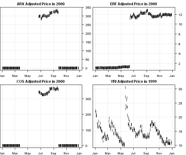
> data.clean(data, min.ratio = 2)	
Removing BNS TRP have less than 756 observations
Abnormal price found for ARX 23-Jun-2000 Ratio : 124.7
Abnormal price found for ARX 26-Sep-2000 Inverse Ratio : 99.4
Abnormal price found for COS 23-Jun-2000 Ratio : 124.1
Abnormal price found for COS 26-Sep-2000 Inverse Ratio : 101.1
Abnormal price found for ERF 14-Jun-2000 Ratio : 7.9
Abnormal price found for YRI 18-Feb-1998 Ratio : 2.1
Abnormal price found for YRI 25-May-1999 Ratio : 3

It is surprising that Bank of Nova Scotia (BNS.TO) has only one year worth of historical data. I also did not find an explanations for jumps in the ARX, COS, ERF during 2000.

Next, I did same analysis for the stocks in the S&P 100 index:

	###############################################################################
	# S&P 100 as of Mar 31 2014
	# http://ca.spindices.com/indices/equity/sp-100
	###############################################################################	
	tickers = spl('MMM,ABT,ABBV,ACN,ALL,MO,AMZN,AXP,AIG,AMGN,APC,APA,AAPL,T,BAC,BAX,BRK.B,BIIB,BA,BMY,COF,CAT,CVX,CSCO,C,KO,CL,CMCSA,COP,COST,CVS,DVN,DOW,DD,EBAY,EMC,EMR,EXC,XOM,FB,FDX,F,FCX,GD,GE,GM,GILD,GS,GOOG,HAL,HPQ,HD,HON,INTC,IBM,JNJ,JPM,LLY,LMT,LOW,MA,MCD,MDT,MRK,MET,MSFT,MDLZ,MON,MS,NOV,NKE,NSC,OXY,ORCL,PEP,PFE,PM,PG,QCOM,RTN,SLB,SPG,SO,SBUX,TGT,TXN,BK,TWX,FOXA,UNP,UPS,UTX,UNH,USB,VZ,V,WMT,WAG,DIS,WFC')
	tickers.suffix = ''

	data <- new.env()
	for(ticker in tickers)
		data[[ticker]] = getSymbols(paste0(ticker, tickers.suffix), src = 'yahoo', from = '1980-01-01', auto.assign = F)

	###############################################################################
	# Plot Abnormal Series
	###############################################################################    
	layout(matrix(1:4,2))	
	plota(data$AAPL$Adjusted['2000'], type='p', pch='|', main='AAPL Adjusted Price in 2000')	
	plota(data$AIG$Adjusted['2008'], type='p', pch='|', main='AIG Adjusted Price in 2008')	
	plota(data$FDX$Adjusted['1982'], type='p', pch='|', main='1982 Adjusted Price in 1982')	

	###############################################################################
	# Clean data
	###############################################################################
	data.clean(data, min.ratio = 2)	

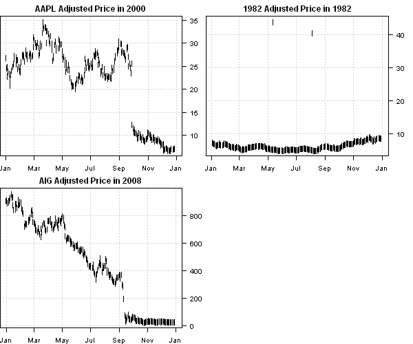
> data.clean(data, min.ratio = 2)	
Removing ABBV FB have less than 756 observations
Abnormal price found for AAPL 29-Sep-2000 Inverse Ratio : 2.1
Abnormal price found for AIG 15-Sep-2008 Inverse Ratio : 2.6
Abnormal price found for FDX 13-May-1982 Ratio : 8
Abnormal price found for FDX 06-Aug-1982 Ratio : 7.8
Abnormal price found for FDX 14-May-1982 Inverse Ratio : 8
Abnormal price found for FDX 09-Aug-1982 Inverse Ratio : 8

I first thought that September 29th, 2000 drop in AAPL was an data error; however, I found following news item: Apple bruises tech sector, September 29, 2000: 4:33 p.m. ET Computer maker’s warning weighs on hardware, chip stocks; Nasdaq tumbles.

So working with data requires a bit of data manipulation and a bit of detective works. Please, always have a look at the data before running any back-tests or making any conclusions.

Capturing Intraday data, Backup plan

In the Capturing Intraday data post, I outlined steps to setup your own process to capture Intraday data. But what do you do if you missed some data points due for example internet being down or due to power outage your server was re-started. To fill up the gaps in the Intraday data, you could get up to 10 day historical Intraday data from Google finance.

I created a wrapper function for Google finance, getSymbol.intraday.google() function in data.r at github, to download historical Intrday quotes. For example,

##############################################################################
# Load Systematic Investor Toolbox (SIT)
# https://systematicinvestor.wordpress.com/systematic-investor-toolbox/
###############################################################################
setInternet2(TRUE)
con = gzcon(url('http://www.systematicportfolio.com/sit.gz', 'rb'))
    source(con)
close(con)

    #*****************************************************************
    # Load Intraday data
    #****************************************************************** 
	data = getSymbol.intraday.google('GOOG', 'NASDAQ', 60, '5d')
	last(data, 10)
	plota(data, type='candle', main='Google Intraday prices')

> last(data, 10)
                       Open    High     Low    Close Volume
2014-03-28 15:52:00 1119.10 1119.61 1119.10 1119.610   4431
2014-03-28 15:53:00 1119.30 1119.30 1118.75 1118.805   3954
2014-03-28 15:54:00 1119.31 1119.45 1119.18 1119.340   5702
2014-03-28 15:55:00 1119.17 1119.40 1119.00 1119.340   8907
2014-03-28 15:56:00 1119.19 1119.35 1119.18 1119.190  11882
2014-03-28 15:57:00 1119.30 1119.30 1119.02 1119.270   6298
2014-03-28 15:58:00 1119.25 1119.35 1119.15 1119.265  10542
2014-03-28 15:59:00 1119.38 1119.49 1118.82 1119.250  29496
2014-03-28 16:00:00 1120.15 1120.15 1119.15 1119.380  71518
2014-03-28 16:01:00 1120.15 1120.15 1120.15 1120.150      0

So if your Intraday capture process failed, you can rely on Google fiance data to fill up the gaps.