November | 2012 | Systematic Investor

Extending Commodity time series

November 22, 2012 systematicinvestor 1 comment

I want to follow up with Extending Gold time series post by showing how we can extend Commodity time series. Most Commodity ETFs began trading in 2006, please see the List of Commodity ETFs page. I will use DBC – PowerShares DB Commodity Fund, one on the most liquid Commodity ETFs as my proxy for Commodity time series.

Unfortunately the historical data for the underlying index for the DBC – PowerShares DB Commodity Fund is not publicly available. Instead I will use Thomson Reuters/Jefferies CRB Index to extend DBC – PowerShares DB Commodity Fund time series.

I created a helper function get.CRB() function in data.r at github to download and extract index information. Please note that I used gdata package to read index data and you might need local Perl available to make it work. There is a great tutorial on setting everything up at How to read an excel file (dot xls and dot xlsx) into a data frame with r: gdata and perl post.

Now let’s plot the CRB index and a few Commodity ETFs side by side to visual check the similarity:

###############################################################################
# Load Systematic Investor Toolbox (SIT)
# https://systematicinvestor.wordpress.com/systematic-investor-toolbox/
###############################################################################
setInternet2(TRUE)
con = gzcon(url('http://www.systematicportfolio.com/sit.gz', 'rb'))
    source(con)
close(con)

	#*****************************************************************
	# Load historical data
	#****************************************************************** 	
	load.packages('quantmod')		
	CRB = get.CRB()
		
	tickers = spl('GSG,DBC')		
	getSymbols(tickers, src = 'yahoo', from = '1970-01-01')
	
	#*****************************************************************
	# Compare different indexes
	#****************************************************************** 	
	out = na.omit(merge(Ad(CRB), Ad(GSG), Ad(DBC)))
		colnames(out) = spl('CRB,GSG,DBC')
	temp = out / t(repmat(as.vector(out[1,]),1,nrow(out)))
		
	# Plot side by side
	layout(1:2, heights=c(4,1))
	plota(temp, ylim=range(temp))
		plota.lines(temp[,1],col=1)
		plota.lines(temp[,2],col=2)
		plota.lines(temp[,3],col=3)
	plota.legend(colnames(temp),1:3)
		
	# Plot correlation table
	temp = compute.cor(temp / mlag(temp)- 1, 'pearson')
			temp[] = plota.format(100 * temp, 0, '', '%')
	plot.table(temp)

The CRB index performed similar to Commodity ETFs; its not the exact replica, but will do given the lack of public historical data for Commodity index.

Next let’s extend the DBC’s time series with CRB index and use it for a simple equal weight strategy:

	#*****************************************************************
	# Create simple equal weight back-test
	#****************************************************************** 
	tickers = spl('GLD,DBC,TLT')

	data <- new.env()
	getSymbols(tickers, src = 'yahoo', from = '1980-01-01', env = data, auto.assign = T)
		for(i in ls(data)) data[[i]] = adjustOHLC(data[[i]], use.Adjusted=T)
		
		# extend Gold and Commodity time series
		data$GLD = extend.GLD(data$GLD)	
		data$DBC = extend.data(data$DBC, get.CRB(), scale=T)
			
	bt.prep(data, align='remove.na')
 
	#*****************************************************************
	# Code Strategies
	#******************************************************************
	prices = data$prices      
	n = ncol(prices)
  
	# find period ends
	period.ends = endpoints(prices, 'months')
		period.ends = period.ends[period.ends > 0]
        
	models = list()
   
	#*****************************************************************
	# Equal Weight
	#******************************************************************
	data$weight[] = NA
		data$weight[period.ends,] = ntop(prices[period.ends,], n)   
	models$equal.weight = bt.run.share(data, clean.signal=F)
    
	#*****************************************************************
	# Create Report
	#******************************************************************       
	plotbt.custom.report.part1(models)       
	plotbt.custom.report.part2(models)

By extending DBC’s and GLD’s time series, the back-test now goes back to the July 2002, the TLT’s first trading date.

To view the complete source code for this example, please have a look at the bt.extend.DBC.test() function in bt.test.r at github.

Categories: R

Regime Detection Pitfalls

November 15, 2012 systematicinvestor Leave a comment

Today, I want to address some questions that I was getting regarding the Regime Detection post. In the Regime Detection post I showed an example based on the simulated data, and some of you tried to apply this example to actual stocks.

There is one big problem that you have to be aware in designing the trading system that uses Regime Detection. Let me demonstrate with a simple example.

Let’s say we used 10 years of daily returns of SPY to train our model (2 regimes: Bull and Bear). Next let’s test a strategy that goes long in the Bull regime and stays in cash in the Bear regime using the out of sample data. I thank you Michael Guan at systematicedge.wordpress.com for asking this question.

###############################################################################
# Load Systematic Investor Toolbox (SIT)
# https://systematicinvestor.wordpress.com/systematic-investor-toolbox/
###############################################################################
setInternet2(TRUE)
con = gzcon(url('http://www.systematicportfolio.com/sit.gz', 'rb'))
    source(con)
close(con)

	#*****************************************************************
	# Load historical data
	#****************************************************************** 
	load.packages('quantmod')	
	data <- new.env()
	getSymbols('SPY', src = 'yahoo', from = '1970-01-01', env = data, auto.assign = T)
		data$SPY = adjustOHLC(data$SPY, use.Adjusted=T)							
	bt.prep(data)
	
	#*****************************************************************
	# Setup
	#****************************************************************** 		
	nperiods = nrow(data$prices)

	models = list()
	
	rets = ROC(Ad(data$SPY))
		rets[1] = 0
	
	# use 10 years: 1993:2002 for training	
	in.sample.index = '1993::2002'
	out.sample.index = '2003::'
		
	in.sample = rets[in.sample.index]
	out.sample = rets[out.sample.index]
	out.sample.first.date = nrow(in.sample) + 1

	#*****************************************************************
	# Fit Model
	#****************************************************************** 		
	load.packages('RHmm')	
	fit = HMMFit(in.sample, nStates=2)
	
	# find states
	states.all = rets * NA
	states.all[] = viterbi(fit, rets)$states
			
	#*****************************************************************
	# Code Strategies
	#****************************************************************** 
	data$weight[] = NA
		data$weight[] = iif(states.all == 1, 0, 1)
		data$weight[in.sample.index] = NA
	models$states.all = bt.run.share(data)

	# create plot
	plotbt.custom.report.part1(models)

These results are too good to be true for such a simple strategy. You have tripped your investment in 10 years with minimum draw-down. So there is the problem?

The Viterbi algorithm uses all data to compute the most likely sequence of states. I.e. In the code above, we passed the returns for all dates to the Viterbi algorithm. Hence, for example, the Viterbi algorithm might use data in 2008 to determine states in 2007. This is a big problem, that we can address using a rolling window approach. Unfortunately, the accuracy of our predictions and strategy returns go down.

	#*****************************************************************
	# Find problem - results are too good
	#****************************************************************** 		
	# The viterbi function need to see all data to compute the most likely sequence of states
	# http://en.wikipedia.org/wiki/Viterbi_algorithm
	
	# We can use expanding window to determine the states
	states.win1 = states.all * NA
	for(i in out.sample.first.date:nperiods) {
		states.win1[i] = last(viterbi(fit, rets[1:i])$states)
		if( i %% 100 == 0) cat(i, 'out of', nperiods, '\n')
	}
	
	# Or we can refit model over expanding window as suggested in the
	# Regime Shifts: Implications for Dynamic Strategies by M. Kritzman, S. Page, D. Turkington
	# Out-of-Sample Analysis, page 8
	initPoint = fit$HMM
	states.win2 = states.all * NA
	for(i in out.sample.first.date:nperiods) {
		fit2 = HMMFit(rets[2:i], nStates=2, control=list(init='USER', initPoint = initPoint))
			initPoint = fit2$HMM
		states.win2[i] = last(viterbi(fit2, rets[2:i])$states)
		if( i %% 100 == 0) cat(i, 'out of', nperiods, '\n')
	}

	#*****************************************************************
	# Plot States
	#****************************************************************** 			
	layout(1:3)
	col = col.add.alpha('white',210)
	plota(states.all[out.sample.index], type='s', plotX=F)
		plota.legend('Implied States based on all data', x='center', bty='o', bg=col, box.col=col,border=col,fill=col,cex=2)
	plota(states.win1[out.sample.index], type='s')
		plota.legend('Implied States based on rolling window', x='center', bty='o', bg=col, box.col=col,border=col,fill=col,cex=2)
	plota(states.win2[out.sample.index], type='s')
		plota.legend('Implied States based on rolling window(re-fit)', x='center', bty='o', bg=col, box.col=col,border=col,fill=col,cex=2)

The states change more often using the rolling window approach. We probably can add a filter that allows the state change only it is confirmed by certain number of observations. I.e. delayed state change, let’s keep it for another post.

Let’s just see the impact of the rolling window approach on the back-test results:

	#*****************************************************************
	# Code Strategies
	#****************************************************************** 		
	data$weight[] = NA
		data$weight[] = iif(states.win1 == 1, 0, 1)
		data$weight[in.sample.index] = NA
	models$states.win1 = bt.run.share(data)
		
	data$weight[] = NA
		data$weight[] = iif(states.win2 == 1, 0, 1)
		data$weight[in.sample.index] = NA
	models$states.win2 = bt.run.share(data)

	#*****************************************************************
	# Create report
	#****************************************************************** 			
	plotbt.custom.report.part1(models)

As expected, it is quite hard to apply Regime Detection to stocks.

To view the complete source code for this example, please have a look at the bt.regime.detection.pitfalls.test() function in bt.test.r at github.

Categories: R

Simulating Multiple Asset Paths in R

November 6, 2012 systematicinvestor Leave a comment

I recently came across the Optimal Rebalancing Strategy Using Dynamic Programming for Institutional Portfolios by W. Sun, A. Fan, L. Chen, T. Schouwenaars, M. Albota paper that examines the cost of different rebablancing methods. For example, one might use calendar rebalancing: i.e. rebalance every month / quarter / year. Or one might use threshold rebalancing: i.e. rebalance only if asset weights break out from a certain band around the policy mix, say 3%.

To investigate the cost of the different rebalancing methods, authors run 10,000 simulations. Today, I want to show how to simulate asset price paths given the expected returns and covariances. I will assume that prices follow the Geometric Brownian Motion. Also I will show a simple application of Monte Carlo option pricing. In the next post I will evaluate the cost of different rebalancing methods.

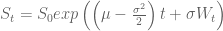
Let’s assume that a stock price can be described by the stochastic differential equation:

$dS_{t}=\mu S_{t}dt+\sigma S_{t}dW_{t}$

where $\mu$ is the expected annual return of the underlying asset, $\sigma$ is the annualized volatility, and $W_{t}$ is a Brownian Motion. This stochastic differential equation has the following solution

$S_{t}=S_{0}exp\left(\left(\mu - \frac{\sigma^{2}}{2}\right)t+\sigma W_{t}\right)$

which I implemented in the asset.paths() function. The asset.paths() function is based on the Simulating Multiple Asset Paths in MATLAB code in Matlab.

asset.paths <- function(s0, mu, sigma, 
	nsims = 10000, 
	periods = c(0, 1)	# time periods at which to simulate prices
) 
{
	s0 = as.vector(s0)
	nsteps = len(periods)
	dt = c(periods[1], diff(periods))
	
	if( len(s0) == 1 ) {
		drift = mu - 0.5 * sigma^2
		if( nsteps == 1 ) {
			s0 * exp(drift * dt + sigma * sqrt(dt) * rnorm(nsims))
		} else {
			temp = matrix(exp(drift * dt + sigma * sqrt(dt) * rnorm(nsteps * nsims)), nc=nsims)
			for(i in 2:nsteps) temp[i,] = temp[i,] * temp[(i-1),]
			s0 * temp
		}
	} else {
		require(MASS)
		drift = mu - 0.5 * diag(sigma)
		n = len(mu)
		
		if( nsteps == 1 ) {
			s0 * exp(drift * dt + sqrt(dt) * t(mvrnorm(nsims, rep(0, n), sigma)))
		} else {
			temp = array(exp(as.vector(drift %*% t(dt)) + t(sqrt(dt) * mvrnorm(nsteps * nsims, rep(0, n), sigma))), c(n, nsteps, nsims))
			for(i in 2:nsteps) temp[,i,] = temp[,i,] * temp[,(i-1),]
			s0 * temp
		}
	}
}

Next let’s visualize some simulation asset paths:

###############################################################################
# Load Systematic Investor Toolbox (SIT)
# https://systematicinvestor.wordpress.com/systematic-investor-toolbox/
###############################################################################
setInternet2(TRUE)
con = gzcon(url('http://www.systematicportfolio.com/sit.gz', 'rb'))
    source(con)
close(con)

	#*****************************************************************
	# Plot some price paths
	#******************************************************************  
	S = c(100,105)
	X = 98
	Time = 0.5
	r = 0.05
	sigma = c(0.11,0.16)
	rho = 0.63
	N = 10000

	# Single Asset for 10 years
	periods = 0:10
	prices = asset.paths(S[1], r, sigma[1], N, periods = periods)
	
	# plot
	matplot(prices[,1:100], type='l', xlab='Years', ylab='Prices',
		main='Selected Price Paths')
	
		
	# Multiple Assets for 10 years
	periods = 0:10
	cov.matrix = sigma%*%t(sigma) * matrix(c(1,rho,rho,1),2,2)
	prices = asset.paths(S, c(r,r), cov.matrix, N, periods = periods)

	# plot
	layout(1:2)
	matplot(prices[1,,1:100], type='l', xlab='Years', ylab='Prices',
		main='Selected Price Paths for Asset 1')
	matplot(prices[2,,1:100], type='l', xlab='Years', ylab='Prices',
		main='Selected Price Paths for Asset 2')

Next, let’s look at examples of Monte Carlo option pricing using asset.paths() function in random.r at github.

	#*****************************************************************
	# Price European Call Option
	#******************************************************************  
	load.packages('fOptions')

	# Black–Scholes
	GBSOption(TypeFlag = "c", S = S[1], X = X, Time = Time, r = r, b = r, sigma = sigma[1])
	
	# Monte Carlo simulation	
	N = 1000000	
	prices = asset.paths(S[1], r, sigma[1], N, periods = Time)
		future.payoff = pmax(0, prices - X)
		discounted.payoff = future.payoff * exp(-r * Time)
	# option price
	mean(discounted.payoff) 

	#*****************************************************************
	# Price Asian Call Option
	#******************************************************************  
	load.packages('fExoticOptions')

	Time = 1/12

	# Approximation
	TurnbullWakemanAsianApproxOption(TypeFlag = "c", S = S[1], SA = S[1], 
  		X = X, Time = Time, time = Time, tau = 0 , r = r, b = r, sigma = sigma[1])
		
	# Monte Carlo simulation		
	N = 100000
	periods = seq(0,Time,1/360)
		n = len(periods)
	prices = asset.paths(S[1], r, sigma[1], N, periods = periods)
		future.payoff = pmax(0, colSums(prices)/n - X)
		discounted.payoff = future.payoff * exp(-r * Time)
	# option price
	mean(discounted.payoff) 

	#*****************************************************************
	# Price Basket Option
	#******************************************************************  
	
	Time = 0.5
	
	# Approximation
	TwoRiskyAssetsOption(TypeFlag = "cmax", S1 = S[1], S2 = S[2],
		X = X, Time = Time, r = r, b1 = r, b2 = r,
		sigma1 = sigma[1], sigma2 = sigma[2], rho = rho)
	
	# Monte Carlo simulation		
	N = 100000
	cov.matrix = sigma%*%t(sigma) * matrix(c(1,rho,rho,1),2,2)
	prices = asset.paths(S, c(r,r), sigma = cov.matrix, N, periods = Time)
		future.payoff = pmax(0, apply(prices,2,max) - X)
		discounted.payoff = future.payoff * exp(-r * Time)
	# option price
	mean(discounted.payoff) 

	#*****************************************************************
	# Price Asian Basket Option
	#******************************************************************  
	
	Time = 1/12
	
	# Monte Carlo simulation		
	N = 10000
	periods = seq(0,Time,1/360)
		n = len(periods)
	
	prices = asset.paths(S, c(r,r), sigma = cov.matrix, N, periods = periods)
		future.payoff = pmax(0, colSums(apply(prices,c(2,3),max))/n - X)
		discounted.payoff = future.payoff * exp(-r * Time)
	# option price
	mean(discounted.payoff)

Please note that Monte Carlo option pricing requireies many simulations to converge to the option price. It takes longer as we increase number of simulations or number of time periods or number of assets. On the positive side, it provides a viable alternative to simulating difficult problems that might not be solved analytically.

In the next post I will look at the cost of different rebalancing methods.

To view the complete source code for this example, please have a look at the asset.paths.test() function in random.r at github.

Categories: R, Risk Measures

Regime Detection

November 1, 2012 systematicinvestor 7 comments

Regime Detection comes handy when you are trying to decide which strategy to deploy. For example there are periods (regimes) when Trend Following strategies work better and there are periods when Mean Reversion strategies work better. Today I want to show you one way to detect market Regimes.

To detect market Regimes, I will fit a Hidden Markov Regime Switching Model on the set of simulated data (i.e. Bull / Bear market environments) I will use the excellent example from the Markov Regime Switching Models in MATLAB post and adapt it to R.

The idea behind using the Regime Switching Models to identify market states is that market returns might have been drawn from 2 or more distinct distributions. As a base case, for example, we may suppose that market returns are samples from one normal distribution N(mu, sigma) i.e.

Returns = mu + e, e ~ N(0, sigma)

Next we may suppose that market returns are samples from two normal distributions (i.e. returns during Bull market may be ~ N(mu.Bull, sigma.Bull) and returns during Bear market may be N(mu.Bear , sigma.Bear) i.e.

Returns = mu + e, e ~ N(0, sigma) 
mu = mu.Bull for Bull regime and mu.Bear for Bear regime and
sigma= sigma.Bull for Bull regime and sigma.Bear for Bear regime

Fortunately we do not have to fit regimes by hand, there is the RHmm package for Hidden Markov Models at CRAN that uses the Baum-Welch algorithm to fit Hidden Markov Models.

Next, let follow the steps from the Markov Regime Switching Models in MATLAB post.

###############################################################################
# Load Systematic Investor Toolbox (SIT)
# https://systematicinvestor.wordpress.com/systematic-investor-toolbox/
###############################################################################
setInternet2(TRUE)
con = gzcon(url('http://www.systematicportfolio.com/sit.gz', 'rb'))
    source(con)
close(con)

	#*****************************************************************
	# Generate data as in the post
	#****************************************************************** 
	bull1 = rnorm( 100, 0.10, 0.15 )
	bear  = rnorm( 100, -0.01, 0.20 )
	bull2 = rnorm( 100, 0.10, 0.15 )
	true.states = c(rep(1,100),rep(2,100),rep(1,100))
	returns = c( bull1, bear,  bull2 )


	# find regimes
	load.packages('RHmm')

	y=returns
	ResFit = HMMFit(y, nStates=2)
	VitPath = viterbi(ResFit, y)

	#Forward-backward procedure, compute probabilities
	fb = forwardBackward(ResFit, y)

	# Plot probabilities and implied states
	layout(1:2)
	plot(VitPath$states, type='s', main='Implied States', xlab='', ylab='State')
	
	matplot(fb$Gamma, type='l', main='Smoothed Probabilities', ylab='Probability')
		legend(x='topright', c('State1','State2'),  fill=1:2, bty='n')

The first chart shows states (1/2) determined by the model. The second chart shows the probability of being in each state.

Next, let’s generate some additional data and see if the model is able to identify the regimes

	#*****************************************************************
	# Add some data and see if the model is able to identify the regimes
	#****************************************************************** 
	bear2  = rnorm( 100, -0.01, 0.20 )
	bull3 = rnorm( 100, 0.10, 0.10 )
	bear3  = rnorm( 100, -0.01, 0.25 )
	y = c( bull1, bear,  bull2, bear2, bull3, bear3 )
	VitPath = viterbi(ResFit, y)$states

	#*****************************************************************
	# Plot regimes
	#****************************************************************** 
	load.packages('quantmod')
	data = xts(y, as.Date(1:len(y)))

	layout(1:3)
		plota.control$col.x.highlight = col.add.alpha(true.states+1, 150)
	plota(data, type='h', plotX=F, x.highlight=T)
		plota.legend('Returns + True Regimes')
	plota(cumprod(1+data/100), type='l', plotX=F, x.highlight=T)
		plota.legend('Equity + True Regimes')
	
		plota.control$col.x.highlight = col.add.alpha(VitPath+1, 150)
	plota(data, type='h', x.highlight=T)
		plota.legend('Returns + Detected Regimes')

The first 300 observations were used to calibrate this model, the next 300 observations were used to see how the model can describe the new infromation. This model does relatively well in our toy example.

To view the complete source code for this example, please have a look at the bt.regime.detection.test() function in bt.test.r at github.

Categories: R

Systematic Investor

Archive

Extending Commodity time series

Regime Detection Pitfalls

Simulating Multiple Asset Paths in R

Regime Detection

Recent Posts

Archives

Categories

Meta

Blogroll