Search Results
Permanent Portfolio – Transaction Cost and better Risk Parity
I want to address comments that were asked in my last post, Permanent Portfolio – Simple Tools, about Permanent Portfolio strategy. Specifically:
- The impact of transaction costs on the perfromance and
- Create a modified version of risk allocation portfolio that distributes weights across 3 asset classes: stocks(SPY), gold(GLD), and treasuries(TLT), and only invests into cash(SHY) to fill the residual portfolio exposure once we scale the SPY/GLD/TLT portfolio to the target volatility
The first point is easy, to incorporate the transaction cost into your back-test just add commission=0.1 parameter to the bt.run.share() function call.For example, to see the dollar allocation strategy perfromance assuming 10c a share commission, use following code:
# original strategy
models$dollar = bt.run.share(data, clean.signal=F)

# assuming 10c a share commissions
models$dollar = bt.run.share(data, commission=0.1, clean.signal=F)
The second point is a bit more work. First, let’s allocate risk across only to 3 asset classes: stocks(SPY), gold(GLD), and treasuries(TLT). Next, let’s scale the SPY/GLD/TLT portfolio to the 7% target volatility. And finally, let’s allocate to cash(SHY) the residual portfolio exposure.
	#*****************************************************************
	# Risk Weighted: allocate only to 3 asset classes: stocks(SPY), gold(GLD), and treasuries(TLT)
	#******************************************************************
	ret.log = bt.apply.matrix(prices, ROC, type='continuous')
	hist.vol = sqrt(252) * bt.apply.matrix(ret.log, runSD, n = 21)
	weight.risk = weight.dollar / hist.vol
		weight.risk$SHY = 0
		weight.risk = weight.risk / rowSums(weight.risk)

	data$weight[] = NA
		data$weight[period.ends,] = weight.risk[period.ends,]
	models$risk = bt.run.share(data, commission=commission, clean.signal=F)

	#*****************************************************************
	# Risk Weighted + 7% target volatility
	#******************************************************************
	data$weight[] = NA
		data$weight[period.ends,] = target.vol.strategy(models$risk,
						weight.risk, 7/100, 21, 100/100)[period.ends,]
	models$risk.target7 = bt.run.share(data, commission=commission, clean.signal=F)

	#*****************************************************************
	# Risk Weighted + 7% target volatility + SHY
	#******************************************************************
	data$weight[] = NA
		data$weight[period.ends,] = target.vol.strategy(models$risk,
						weight.risk, 7/100, 21, 100/100)[period.ends,]

  		cash = 1-rowSums(data$weight)
	    data$weight$SHY[period.ends,] = cash[period.ends]
	models$risk.target7.shy = bt.run.share(data, commission=commission, clean.signal=F)
The modified version of risk allocation portfolio performs well relative to other portfolios even after incorporating the 10c transaction cost.
To view the complete source code for this example, please have a look at the bt.permanent.portfolio3.test() function in bt.test.r at github.
Permanent Portfolio – Simple Tools
I have previously described and back-tested the Permanent Portfolio strategy based on the series of posts at the GestaltU blog. Today I want to show how we can improve the Permanent Portfolio strategy perfromance using following simple tools:
- Volatility targeting
- Risk allocation
- Tactical market filter
First, let’s load the historical prices for the stocks(SPY), gold(GLD), treasuries(TLT), and cash(SHY) and create a quarterly rebalanced Permanent Portfolio strategy using the Systematic Investor Toolbox.
###############################################################################
# Load Systematic Investor Toolbox (SIT)
# https://systematicinvestor.wordpress.com/systematic-investor-toolbox/
###############################################################################
setInternet2(TRUE)
con = gzcon(url('http://www.systematicportfolio.com/sit.gz', 'rb'))
    source(con)
close(con)

	#*****************************************************************
	# Load historical data
	#******************************************************************
	load.packages('quantmod')
	tickers = spl('SPY,TLT,GLD,SHY')

	data <- new.env()
	getSymbols(tickers, src = 'yahoo', from = '1980-01-01', env = data, auto.assign = T)
		for(i in ls(data)) data[[i]] = adjustOHLC(data[[i]], use.Adjusted=T)

		# extend GLD with Gold.PM - London Gold afternoon fixing prices
		data$GLD = extend.GLD(data$GLD)

	bt.prep(data, align='remove.na')

	#*****************************************************************
	# Setup
	#******************************************************************
	prices = data$prices
		n = ncol(prices)

	period.ends = endpoints(prices, 'quarters')
		period.ends = period.ends[period.ends > 0]
		period.ends = c(1, period.ends)


	models = list()


	#*****************************************************************
	# Dollar Weighted
	#******************************************************************
	target.allocation = matrix(rep(1/n,n), nrow=1)
	weight.dollar = ntop(prices, n)

	data$weight[] = NA
		data$weight[period.ends,] = weight.dollar[period.ends,]
	models$dollar = bt.run.share(data, clean.signal=F)
Now let’s create a version of the Permanent Portfolio strategy that targets the 7% annual volatility based on the 21 day look back period.
	#*****************************************************************
	# Dollar Weighted + 7% target volatility
	#******************************************************************
	data$weight[] = NA
		data$weight[period.ends,] = target.vol.strategy(models$dollar,
						weight.dollar, 7/100, 21, 100/100)[period.ends,]
	models$dollar.target7 = bt.run.share(data, clean.signal=F)
Please note that allocating equal dollar amounts to each investment puts more risk allocation to the risky assets. If we want to distribute risk budget equally across all assets we can consider a portfolio based on the equal risk allocation instead of equal capital (dollar) allocation.
	#*****************************************************************
	# Risk Weighted
	#******************************************************************
	ret.log = bt.apply.matrix(prices, ROC, type='continuous')
	hist.vol = sqrt(252) * bt.apply.matrix(ret.log, runSD, n = 21)
	weight.risk = weight.dollar / hist.vol
		weight.risk = weight.risk / rowSums(weight.risk)

	data$weight[] = NA
		data$weight[period.ends,] = weight.risk[period.ends,]
	models$risk = bt.run.share(data, clean.signal=F)
We can also use market filter, for example a 10 month moving average, to control portfolio drawdowns.
	#*****************************************************************
	# Market Filter (tactical): 10 month moving average
	#******************************************************************
	period.ends = endpoints(prices, 'months')
		period.ends = period.ends[period.ends > 0]
		period.ends = c(1, period.ends)

	sma = bt.apply.matrix(prices, SMA, 200)
	weight.dollar.tactical = weight.dollar * (prices > sma)

	data$weight[] = NA
		data$weight[period.ends,] = weight.dollar.tactical[period.ends,]
	models$dollar.tactical = bt.run.share(data, clean.signal=F)
Finally, let’s combine market filter and volatility targeting:
	#*****************************************************************
	# Tactical + 7% target volatility
	#******************************************************************
	data$weight[] = NA
		data$weight[period.ends,] = target.vol.strategy(models$dollar.tactical,
						weight.dollar.tactical, 7/100, 21, 100/100)[period.ends,]
	models$dollar.tactical.target7 = bt.run.share(data, clean.signal=F)


	#*****************************************************************
	# Create Report
	#******************************************************************
	plotbt.custom.report.part1(models)

	plotbt.strategy.sidebyside(models)
The final portfolio that combines market filter and volatility targeting is a big step up from the original Permanent Portfolio strategy: the returns are a bit down, but draw-downs are cut in half.
To view the complete source code for this example, please have a look at the bt.permanent.portfolio2.test() function in bt.test.r at github.
Permanent Portfolio
First, just a quick update: I’m moving the release date of the SIT package a few months down the road, probably in November.
Now back to the post. Recently I came across a series of interesting posts about the Permanent Portfolio at the GestaltU blog. Today I want to show you how to back-test the Permanent Portfolio using the Systematic Investor Toolbox.
The simple version of the Permanent Portfolio consists of equal allocations to stocks(SPY), gold(GLD), treasuries(TLT), and cash(SHY). [25% allocation each] The portfolio is rebalanced once a year if any allocation breaks out from the 15% – 35% range.
###############################################################################
# Load Systematic Investor Toolbox (SIT)
# https://systematicinvestor.wordpress.com/systematic-investor-toolbox/
###############################################################################
setInternet2(TRUE)
con = gzcon(url('http://www.systematicportfolio.com/sit.gz', 'rb'))
    source(con)
close(con)

	#*****************************************************************
	# Load historical data
	#******************************************************************
	load.packages('quantmod')
	tickers = spl('SPY,TLT,GLD,SHY')

	data <- new.env()
	getSymbols(tickers, src = 'yahoo', from = '1980-01-01', env = data, auto.assign = T)
		for(i in ls(data)) data[[i]] = adjustOHLC(data[[i]], use.Adjusted=T)

		# extend GLD with Gold.PM - London Gold afternoon fixing prices
		data$GLD = extend.GLD(data$GLD)

	bt.prep(data, align='remove.na')

	#*****************************************************************
	# Code Strategies
	#******************************************************************
	prices = data$prices
		n = ncol(prices)
		nperiods = nrow(prices)

	# annual
	period.ends = endpoints(prices, 'years')
		period.ends = period.ends[period.ends > 0]
		period.ends.y = c(1, period.ends)

	# quarterly
	period.ends = endpoints(prices, 'quarters')
		period.ends = period.ends[period.ends > 0]
		period.ends.q = c(1, period.ends)

	models = list()

	#*****************************************************************
	# Code Strategies
	#******************************************************************
	target.allocation = matrix(rep(1/n,n), nrow=1)

	# Buy & Hold
	data$weight[] = NA
		data$weight[period.ends.y[1],] = target.allocation
	models$buy.hold = bt.run.share(data, clean.signal=F)

	# Equal Weight Annual
	data$weight[] = NA
		data$weight[period.ends.y,] = ntop(prices[period.ends.y,], n)
	models$equal.weight.y = bt.run.share(data, clean.signal=F)

	# Equal Weight Quarterly
	data$weight[] = NA
		data$weight[period.ends.q,] = ntop(prices[period.ends.q,], n)
	models$equal.weight.q = bt.run.share(data, clean.signal=F)
To rebalance base on the 10% threshold (i.e. portfolio weights breaking out from the 15% – 35% range) I will use bt.max.deviation.rebalancing() function introduced in the Backtesting Rebalancing methods post.
	#*****************************************************************
	# Rebalance based on threshold
	#******************************************************************
	# Rebalance only when threshold is broken
	models$threshold.y = bt.max.deviation.rebalancing(data, models$buy.hold, target.allocation, 10/100, 0, period.ends = period.ends.y)

	# Rebalance only when threshold is broken
	models$threshold.q = bt.max.deviation.rebalancing(data, models$buy.hold, target.allocation, 10/100, 0, period.ends = period.ends.q)

	#*****************************************************************
	# Create Report
	#******************************************************************
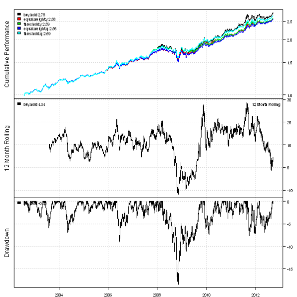
	plotbt.custom.report.part1(models)

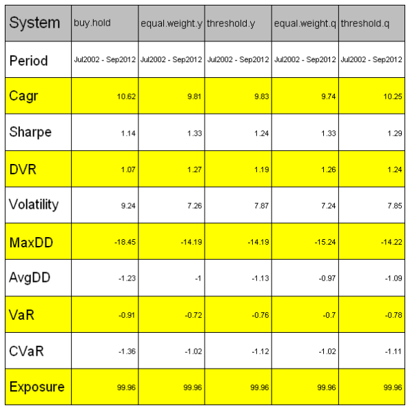
	plotbt.strategy.sidebyside(models)

	# Plot Portfolio Turnover for each Rebalancing method
	layout(1:2)
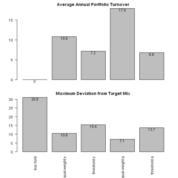
	barplot.with.labels(sapply(models, compute.turnover, data), 'Average Annual Portfolio Turnover', F)
	barplot.with.labels(sapply(models, compute.max.deviation, target.allocation), 'Maximum Deviation from Target Mix')
The Quarterly rebalancing with 10% threshold produces an attractive portfolio with top performance and low turnover.
To view the complete source code for this example, please have a look at the bt.permanent.portfolio.test() function in bt.test.r at github.
Modeling Couch Potato strategy
I first read about the Couch Potato strategy in the MoneySense magazine. I liked this simple strategy because it was easy to understand and easy to manage. The Couch Potato strategy is similar to the Permanent Portfolio strategy that I have analyzed previously.
The Couch Potato strategy invests money in the given proportions among different types of assets to ensure diversification and rebalances the holdings once a year. For example the Classic Couch Potato strategy is:
- 1) Canadian equity (33.3%)
- 2) U.S. equity (33.3%)
- 3) Canadian bond (33.3%)
I highly recommend reading following online resources to get more information about the Couch Potato strategy:
- MoneySense
- Canadian Couch Potato
- AssetBuilder
Today, I want to show how you can model and monitor the Couch Potato strategy with the Systematic Investor Toolbox.
###############################################################################
# Load Systematic Investor Toolbox (SIT)
# https://systematicinvestor.wordpress.com/systematic-investor-toolbox/
###############################################################################
setInternet2(TRUE)
con = gzcon(url('http://www.systematicportfolio.com/sit.gz', 'rb'))
    source(con)
close(con)


	# helper function to model Couch Potato strategy - a fixed allocation strategy
	couch.potato.strategy <- function
	(
		data.all,
		tickers = 'XIC.TO,XSP.TO,XBB.TO',
		weights = c( 1/3, 1/3, 1/3 ),
		periodicity = 'years',
		dates = '1900::',
		commission = 0.1
	)
	{
		#*****************************************************************
		# Load historical data
		#******************************************************************
		tickers = spl(tickers)
		names(weights) = tickers

		data <- new.env()
		for(s in tickers) data[[ s ]] = data.all[[ s ]]

		bt.prep(data, align='remove.na', dates=dates)

		#*****************************************************************
		# Code Strategies
		#******************************************************************
		prices = data$prices
			n = ncol(prices)
			nperiods = nrow(prices)

		# find period ends
		period.ends = endpoints(data$prices, periodicity)
			period.ends = c(1, period.ends[period.ends > 0])

		#*****************************************************************
		# Code Strategies
		#******************************************************************
		data$weight[] = NA
			for(s in tickers) data$weight[period.ends, s] = weights[s]
		model = bt.run.share(data, clean.signal=F, commission=commission)

		return(model)
	}
The couch.potato.strategy() function creates a periodically rebalanced portfolio for given static allocation.
Next, let’s back-test some Canadian Couch Potato portfolios:
	#*****************************************************************
	# Load historical data
	#******************************************************************
	load.packages('quantmod')
	map = list()
		map$can.eq = 'XIC.TO'
		map$can.div = 'XDV.TO'
		map$us.eq = 'XSP.TO'
		map$us.div = 'DVY'
		map$int.eq = 'XIN.TO'
		map$can.bond = 'XBB.TO'
		map$can.real.bond = 'XRB.TO'
		map$can.re = 'XRE.TO'
		map$can.it = 'XTR.TO'
		map$can.gold = 'XGD.TO'

	data <- new.env()
	for(s in names(map)) {
		data[[ s ]] = getSymbols(map[[ s ]], src = 'yahoo', from = '1995-01-01', env = data, auto.assign = F)
		data[[ s ]] = adjustOHLC(data[[ s ]], use.Adjusted=T)
	}

	#*****************************************************************
	# Code Strategies
	#******************************************************************
	models = list()
		periodicity = 'years'
		dates = '2006::'

	models$classic = couch.potato.strategy(data, 'can.eq,us.eq,can.bond', rep(1/3,3), periodicity, dates)
	models$global = couch.potato.strategy(data, 'can.eq,us.eq,int.eq,can.bond', c(0.2, 0.2, 0.2, 0.4), periodicity, dates)
	models$yield = couch.potato.strategy(data, 'can.div,can.it,us.div,can.bond', c(0.25, 0.25, 0.25, 0.25), periodicity, dates)
	models$growth = couch.potato.strategy(data, 'can.eq,us.eq,int.eq,can.bond', c(0.25, 0.25, 0.25, 0.25), periodicity, dates)

	models$complete = couch.potato.strategy(data, 'can.eq,us.eq,int.eq,can.re,can.real.bond,can.bond', c(0.2, 0.15, 0.15, 0.1, 0.1, 0.3), periodicity, dates)

	models$permanent = couch.potato.strategy(data, 'can.eq,can.gold,can.bond', c(0.25,0.25,0.5), periodicity, dates)

	#*****************************************************************
	# Create Report
	#******************************************************************
	plotbt.custom.report.part1(models)
I have included a few classic Couch Potato portfolios and the Canadian version of the Permanent portfolio. The equity curves speak for themselves: you can call them by the fancy names, but in the end all variations of the Couch Potato portfolios performed similar and suffered a huge draw-down during 2008. The Permanent portfolio did a little better during 2008 bear market.
Next, let’s back-test some US Couch Potato portfolios:
	#*****************************************************************
	# Load historical data
	#******************************************************************
	tickers = spl('VIPSX,VTSMX,VGTSX,SPY,TLT,GLD,SHY')

	data <- new.env()
	getSymbols(tickers, src = 'yahoo', from = '1995-01-01', env = data, auto.assign = T)
		for(i in ls(data)) data[[i]] = adjustOHLC(data[[i]], use.Adjusted=T)

		# extend GLD with Gold.PM - London Gold afternoon fixing prices
		data$GLD = extend.GLD(data$GLD)

	#*****************************************************************
	# Code Strategies
	#******************************************************************
	models = list()
		periodicity = 'years'
		dates = '2003::'

	models$classic = couch.potato.strategy(data, 'VIPSX,VTSMX', rep(1/2,2), periodicity, dates)
	models$margarita = couch.potato.strategy(data, 'VIPSX,VTSMX,VGTSX', rep(1/3,3), periodicity, dates)
	models$permanent = couch.potato.strategy(data, 'SPY,TLT,GLD,SHY', rep(1/4,4), periodicity, dates)

	#*****************************************************************
	# Create Report
	#******************************************************************
	plotbt.custom.report.part1(models)
The US Couch Potato portfolios also suffered huge draw-downs during 2008. The Permanent portfolio hold it ground much better.
It has been written quite a lot about Couch Potato strategy, but looking at different variations I cannot really see much difference in terms of perfromance or draw-downs. Probably that is why in the last few years, I have seen the creation of many new ETFs to address that in one way or another. For example, now we have tactical asset allocation ETFs, minimum volatility ETFs, income ETFs with covered calls overlays.
To view the complete source code for this example, please have a look at the bt.couch.potato.test() function in bt.test.r at github.
Some additional references from the Canadian Couch Potato blog that are worth reading:


